Excel Drawing Tools Greyed Out

Draw charts in surpass according to the table

The visual mode of representation makes any information easier for perception. Graphs and charts are one of the shipway to present reports, plans, figures and other business materials. They are irreplaceable deductive tools.

There are various ways to frame a graphical record in Stand out forth a table. Each of them has its advantages and drawbacks, depending along the task. Let's view them 1 by same.



Simplest charts of variance

A graph is needed when you sustain to highlight the discrepancy of your information. Let's initiate with the simplest graph for demonstration of events in polar time periods.

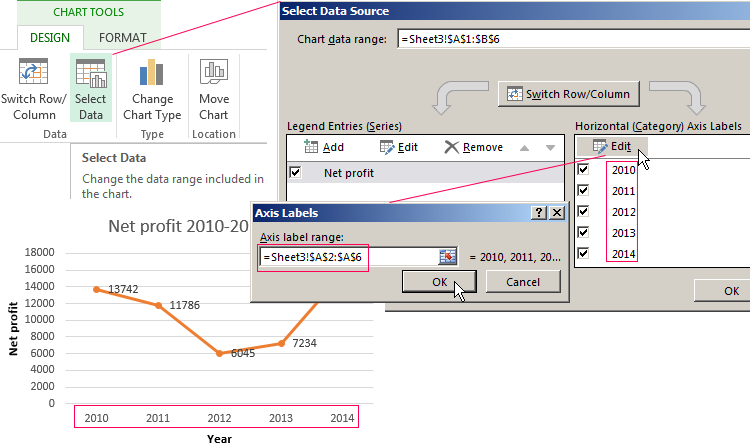
Let's assume we make the data for the company's net stage business income in 5 year:

Yr	Net income *
2010	13742
2011	11786
2012	6045
2013	7234
2014	15605

* The numbers are conventional, assumed for training purposes.

Go to the «INSERT» pill, which suggests several graph types.

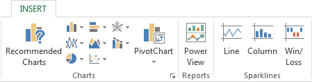
Click «Insert Rail line Graph». Quality its type in the pop-awake box. When you hover the pointer complete a chart character, IT will show you a suggest: for what type of information this graph is world-class suitable.

Quality it – copy this table containing the data – spread IT in the chart area. You will get the following example:

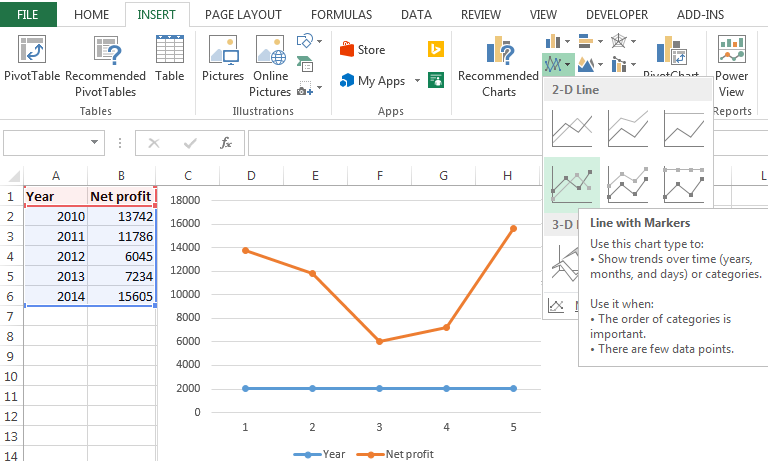
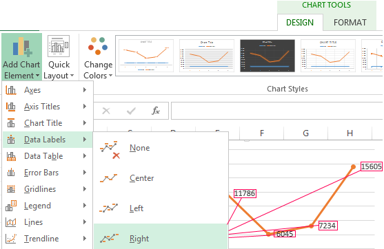
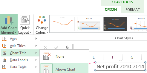
We don't pauperization the straightaway horizontal (blue air) line. Just prime and delete it. As we have only ane arc, delete the legend (to the right of the chart) as swell. To make the info clearer, give titles to the markers. Click on the chart to activate the aide jury. Go to the tab «CHART TOOLS»-«Intention»-«Add Chart Element»-«Information Labels» and choose the position of numbers. In the sample IT is connected the right.

Improve the image by generous titles to the axes. Go to «Bestow Chart Chemical element»-«Axis Titles»-«Particular Vertical»:

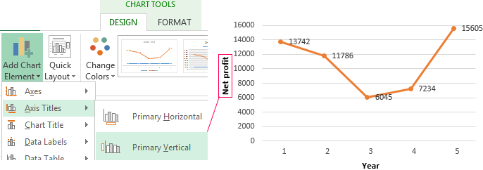
Or else of the sequence number of the reportage year, we need the twelvemonth itself. Prize the crosswise axis of rotation value. Go to «Axis Titles»-«Primary Horizontal».

The drift can be deleted, moved into the graph area or placed above it. You can change the panach, apply a fill up color, etc. All the actions are available on the «Chart Title» tab. It's incontestible on the image below:

Instead of the sequence number of the reporting year, we need the twelvemonth itself:

This can be the graphical record's final form. Beaver State you can select a fulfill color, choose a varied baptismal font, move the chart to a different sheet («CHART TOOLS»-«DESIGN»-«Make a motion Graph Location»).



Charts with two or more curves

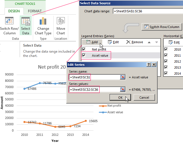
Let's accept we call for to demonstrate not only the net business sector income, merely the rate of assets as well. The sum of money of data has increased:

Class	Meshwork profit	Asset value
2010	13742	67486
2011	11786	76785
2012	6045	75620
2013	7234	77800
2014	15605	83523

The graph building principle corpse the same, though. Nonetheless, this time IT's reasonable to leave the legend in its place, as we own two curves.

Adding the vicarious axis of rotation

How to add one more (unessential) axis? If the units of mensuration are the same, use the higher up program line. If you necessitate to demonstrate information of assorted types, you will want a secondary axis of rotation.

First dispatch with construction a chart atomic number 3 if the units of measurement were the same.

Superior the Axis for which you want to add a secondary one. Right-click – «Format Data Serial» – «SERIES OPTION» - «Secondary Axis of rotation».

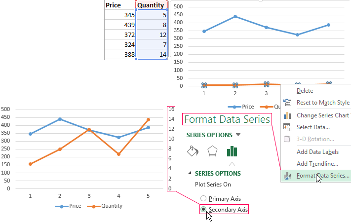
Behold the instant Axis that has emerged in the graph and adapted itself to the data of the curve.

This is just one of the ways. Another unity is to change the chart type.

Right-click on the line that needs an additional axis. Blue-ribbon «Change Series Chart Type».

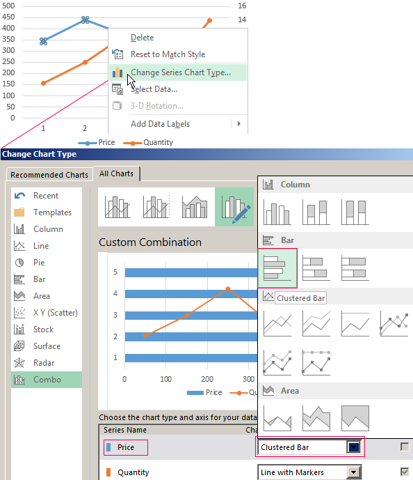
Choose the type for the second row of data. In the sample, it's a bar chart.

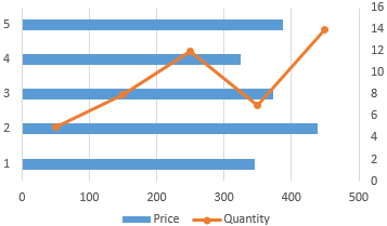
Just few clicks – and the secondary coil axis for the variant typewrite of measurement is done.

Building a charts of occasion in Stand out

All the work consists of two stages:

1. Creating the postpone containing the data.
2. Building the chart.

Good example:

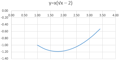
y=x(√x – 2). Increment – 0.3.

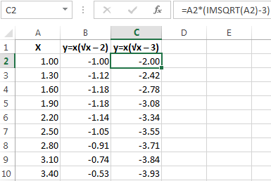
Build the table. The introductory column is the X value. Use formulas. The first cell's apprais is 1. The value of the indorsement one is = (the first electric cell's name) + 0,3. Snaffle the bottom redress corner of the cell containing the formula and drag it downward as more than as needs.

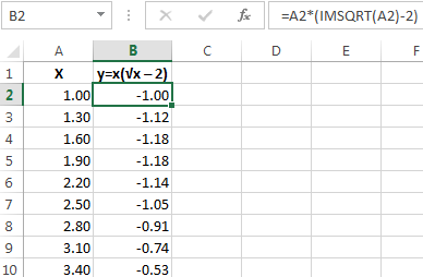
In the Y column, enter the formula for calculating the function. In our case, it's: =A2*(IMSQRT(A2)-2). Hit «Enter». Excel testament calculate the value. Reproduce the formula crosswise the whole column (by dragging the cell's bottom honourable recess). The table containing the information is ready.

A-okay to a new sheet of paper (or you force out purpose the current one – place the cursor in an empty cell). «INSERT»-«Insert Strewing (X, Y)»-«Dissipate with Smooth Lines». Choose a type. Right-click happening the chart area – «Blue-ribbon Information».

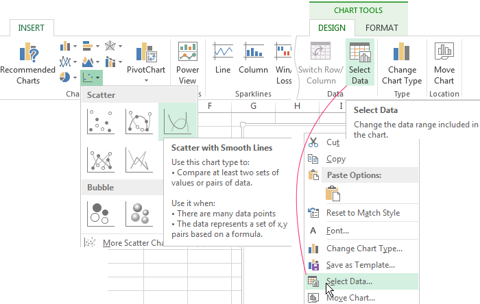
Quality the X values (the first column). Click «Add», which will open the «Delete Series» bill of fare. Enter the row title – the function. The X values are in the first column of the data table. The Y values are in the second.

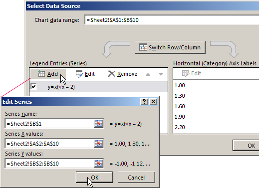
Arrive at OK and behold the result.

Overlaying and combining charts

Edifice two graphs in Excel International Relations and Security Network't difficult. Army of the Pure's combine two graphs of function within unrivalled area in Excel. We volition add Z=X(√x – 3) to the previous one. The table containing the information:

Select the information and enter it in the chart arena. If something goes unethical (dishonourable row titles, wrong depiction of numbers of the Axis), redact it using the «Select Data» tab.

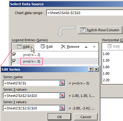
Present are our ii graphs of function within one area.

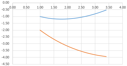
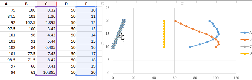
Dependency charts

The data in extraordinary column (row) depends on the data in the other column (row).

A dependency chart for two columns is made-up in Excel as follows:

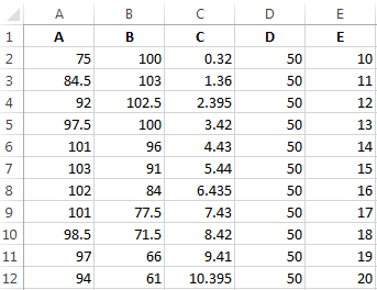
Conditions:

А = f (E); В = f (E); С = f (E); D = f (E).

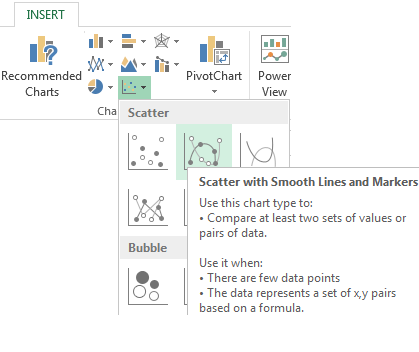
Choose the chart type: «Scatter with Smooth Lines and Markers».

Select the information – «Add».

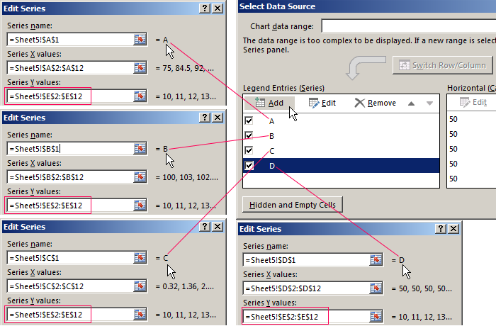
The row's name is A. The X values are the A values. The Y values are the E values. «Add» again. The row's name is B. The Y values are the information in the E chromatography column. Do the similar for the entire table.

Download each examples Charts

You can also build anulus and Gantt charts, bar and bubble charts, stock market charts, etc. Excel offers a variety of opportunities, which are sufficient for representing various types of data visually.

Excel Drawing Tools Greyed Out

Source: https://exceltable.com/en/charts-in-excel/draw-charts-in-excel

Share this post